GLM Logit 的影响度量
基于 GLMInfluence 的草案版本,它也适用于离散 Logit、Probit 和 Poisson,并最终扩展到涵盖时间序列分析以外的大多数模型。
逻辑回归的示例由 Pregibon (1981) 的“Logistic Regression diagnostics”使用,并基于 Finney (1947) 的数据。
GLMInfluence 包含基本的影响度量,但仍然缺少 Pregibon (1981) 中描述的一些度量,例如与偏差和对置信区间的影響有关的度量。
[1]:
import os.path
import pandas as pd
import matplotlib.pyplot as plt

from statsmodels.genmod.generalized_linear_model import GLM
from statsmodels.genmod import families

plt.rc("figure", figsize=(16, 8))
plt.rc("font", size=14)
[2]:
import statsmodels.stats.tests.test_influence

test_module = statsmodels.stats.tests.test_influence.__file__
cur_dir = cur_dir = os.path.abspath(os.path.dirname(test_module))

file_name = "binary_constrict.csv"
file_path = os.path.join(cur_dir, "results", file_name)
df = pd.read_csv(file_path, index_col=0)
[3]:
res = GLM(
    df["constrict"],
    df[["const", "log_rate", "log_volumne"]],
    family=families.Binomial(),
).fit(attach_wls=True, atol=1e-10)
print(res.summary())
                 Generalized Linear Model Regression Results
==============================================================================
Dep. Variable:              constrict   No. Observations:                   39
Model:                            GLM   Df Residuals:                       36
Model Family:                Binomial   Df Model:                            2
Link Function:                  Logit   Scale:                          1.0000
Method:                          IRLS   Log-Likelihood:                -14.614
Date:                Thu, 03 Oct 2024   Deviance:                       29.227
Time:                        15:49:03   Pearson chi2:                     34.2
No. Iterations:                     7   Pseudo R-squ. (CS):             0.4707
Covariance Type:            nonrobust
===============================================================================
                  coef    std err          z      P>|z|      [0.025      0.975]
-------------------------------------------------------------------------------
const          -2.8754      1.321     -2.177      0.029      -5.464      -0.287
log_rate        4.5617      1.838      2.482      0.013       0.959       8.164
log_volumne     5.1793      1.865      2.777      0.005       1.524       8.834
===============================================================================
获取影响度量
GLMResults 具有与 OLSResults 类似的 get_influence 方法,它返回 GLMInfluence 类的实例。此类具有用于检查影响和异常值度量的方法和(缓存)属性。
这些度量基于对删除一个观测结果的结果进行一步近似。一步近似对于较小的变化通常是准确的,但会低估较大变化的大小。即使低估了较大变化,它们仍然清楚地表明了影响性观测结果的影响。
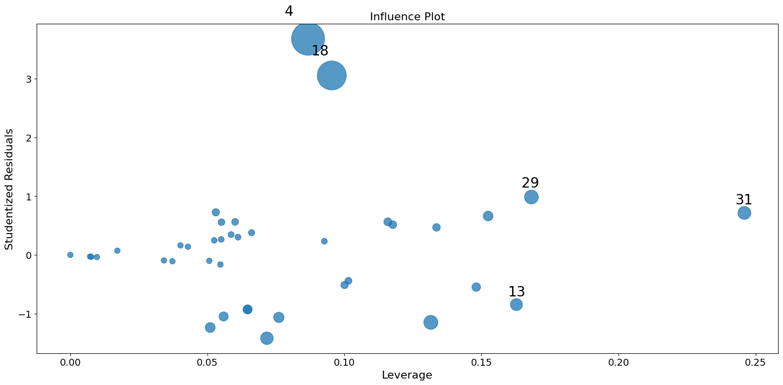
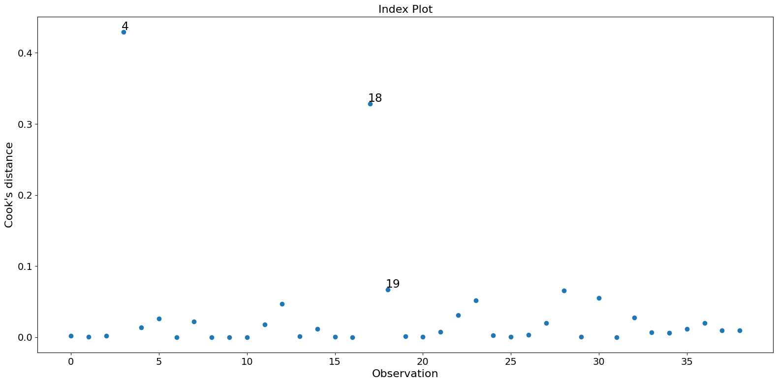
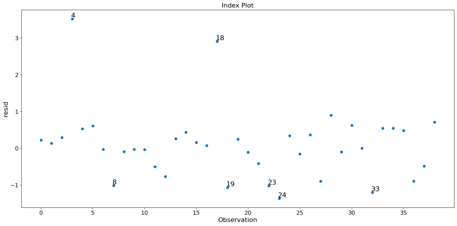
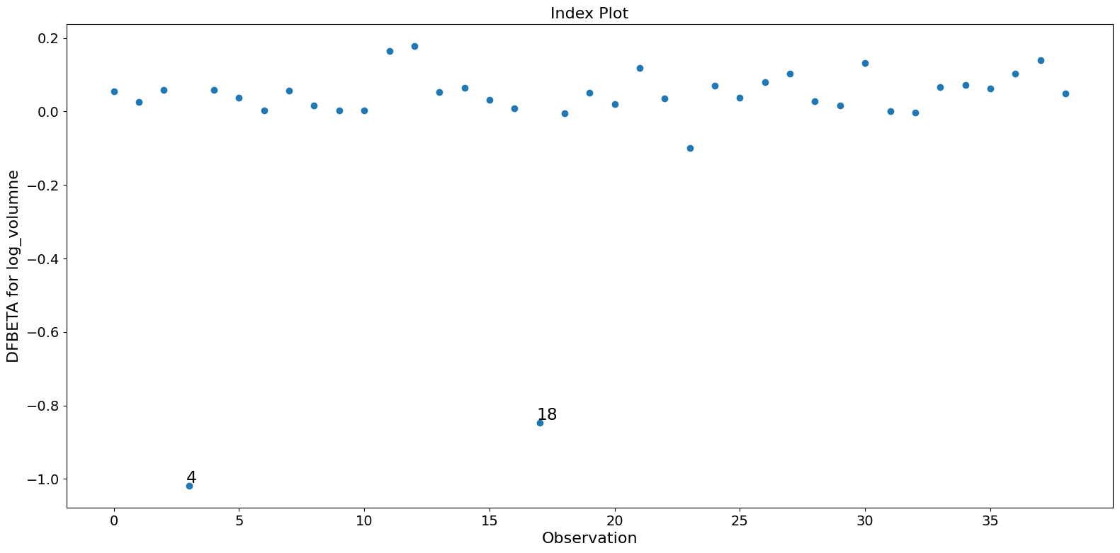
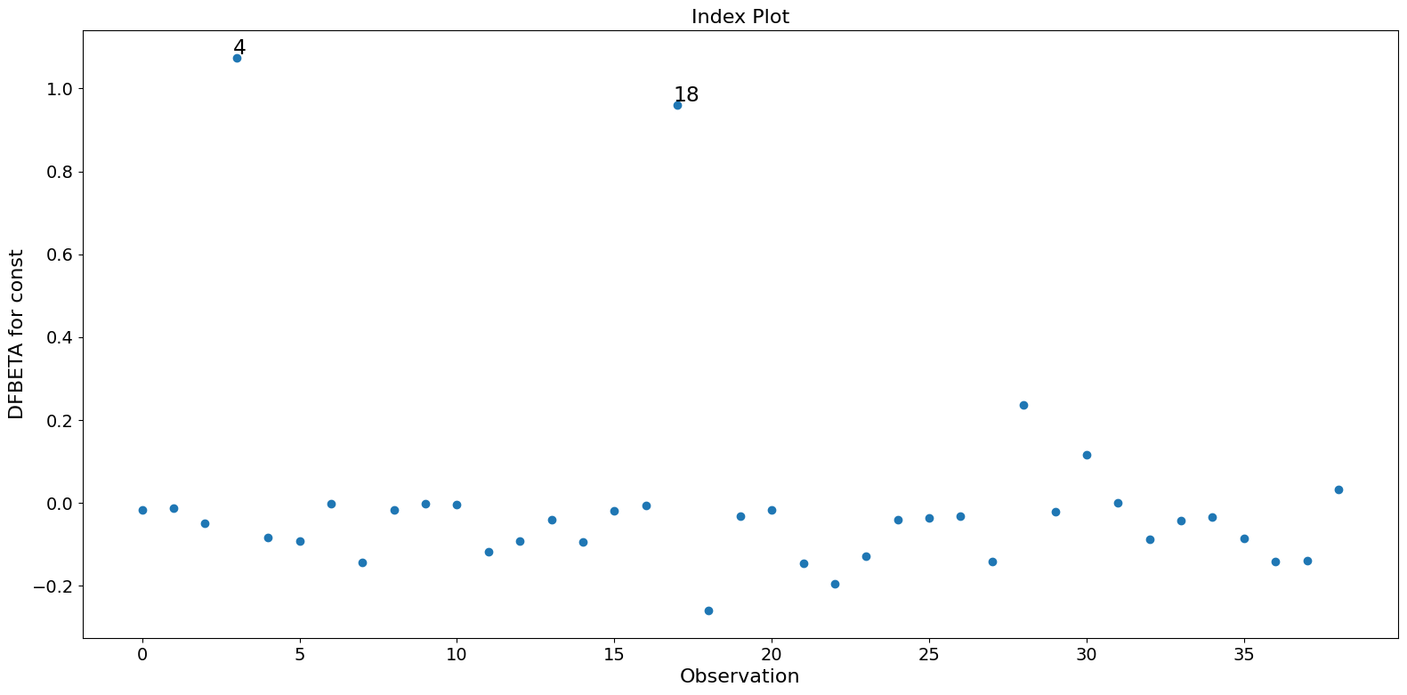
在这个示例中,观测值 4 和 18 具有较大的标准化残差和较大的 Cook 距离,但没有较大的杠杆。观测值 13 具有最大的杠杆,但只有较小的 Cook 距离,没有较大的学生化残差。
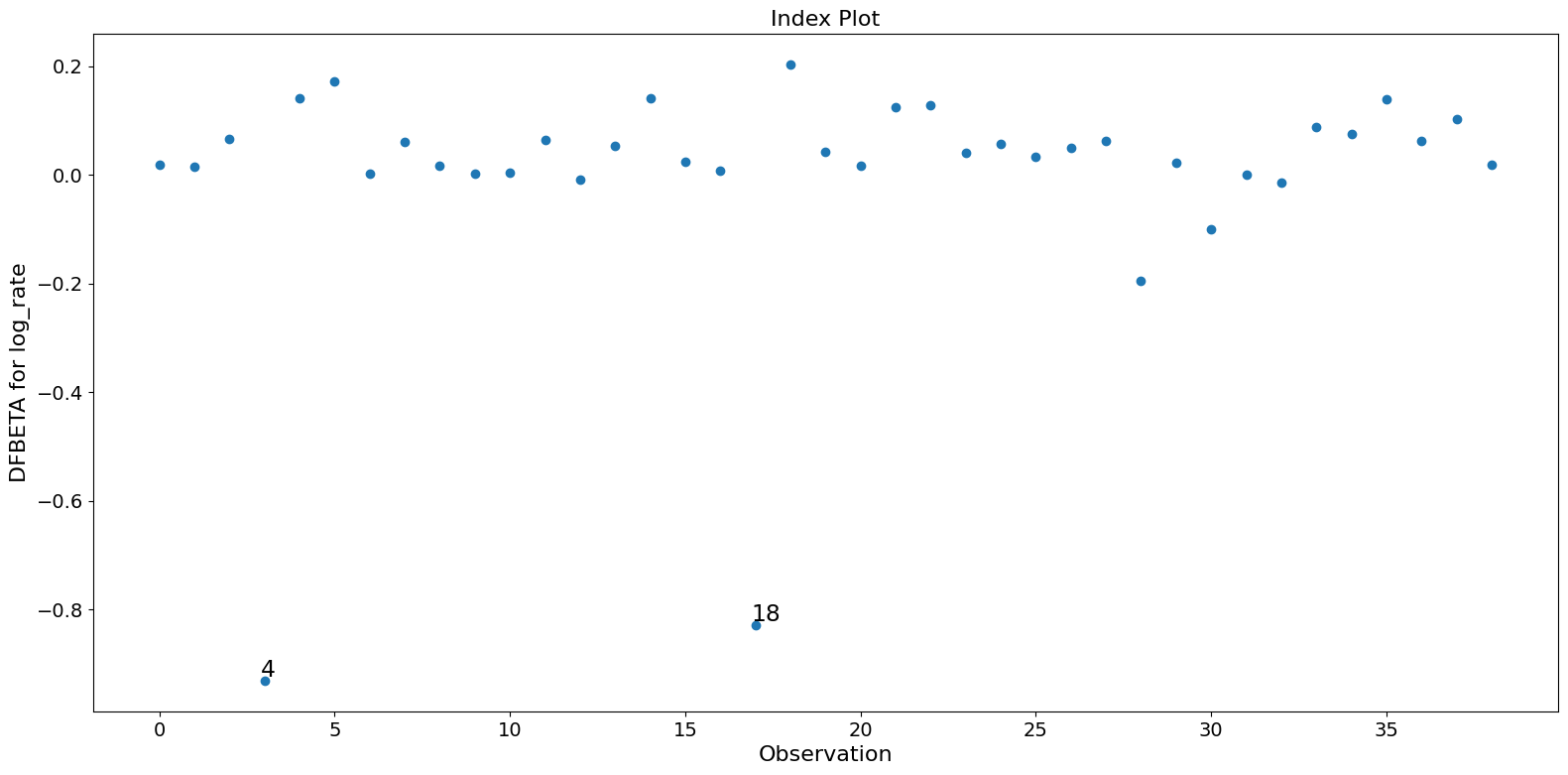
只有两个观测值 4 和 18 对参数估计有很大影响。
[4]:
infl = res.get_influence(observed=False)
[5]:
summ_df = infl.summary_frame()
summ_df.sort_values("cooks_d", ascending=False)[:10]
[5]:
| dfb_const | dfb_log_rate | dfb_log_volumne | cooks_d | standard_resid | hat_diag | dffits_internal | |
|---|---|---|---|---|---|---|---|
| 案例 | |||||||
| 4 | 1.073359 | -0.930200 | -1.017953 | 0.429085 | 3.681352 | 0.086745 | 1.134573 |
| 18 | 0.959508 | -0.827905 | -0.847666 | 0.328152 | 3.055542 | 0.095386 | 0.992197 |
| 19 | -0.259120 | 0.202363 | -0.004883 | 0.066770 | -1.150095 | 0.131521 | -0.447560 |
| 29 | 0.236747 | -0.194984 | 0.028643 | 0.065370 | 0.984729 | 0.168219 | 0.442844 |
| 31 | 0.116501 | -0.099602 | 0.132197 | 0.055382 | 0.713771 | 0.245917 | 0.407609 |
| 24 | -0.128107 | 0.041039 | -0.100410 | 0.051950 | -1.420261 | 0.071721 | -0.394777 |
| 13 | -0.093083 | -0.009463 | 0.177532 | 0.046492 | -0.847046 | 0.162757 | -0.373465 |
| 23 | -0.196119 | 0.127482 | 0.035689 | 0.031168 | -1.065576 | 0.076085 | -0.305786 |
| 33 | -0.088174 | -0.013657 | -0.002161 | 0.027481 | -1.238185 | 0.051031 | -0.287130 |
| 6 | -0.092235 | 0.170980 | 0.038080 | 0.026230 | 0.661478 | 0.152431 | 0.280520 |
[6]:
fig = infl.plot_influence()
fig.tight_layout(pad=1.0)
[7]:
fig = infl.plot_index(y_var="cooks", threshold=2 * infl.cooks_distance[0].mean())
fig.tight_layout(pad=1.0)
[8]:
fig = infl.plot_index(y_var="resid", threshold=1)
fig.tight_layout(pad=1.0)
[9]:
fig = infl.plot_index(y_var="dfbeta", idx=1, threshold=0.5)
fig.tight_layout(pad=1.0)
[10]:
fig = infl.plot_index(y_var="dfbeta", idx=2, threshold=0.5)
fig.tight_layout(pad=1.0)
[11]:
fig = infl.plot_index(y_var="dfbeta", idx=0, threshold=0.5)
fig.tight_layout(pad=1.0)
[ ]:
上次更新:2024 年 10 月 3 日